Wave/Particle duality
It is sometimes claimed that a strange feature of quantum mechanics is “wave/particle duality,” meaning that sometimes that which we call a particle acts like a wave and sometimes acts like a particle. In one sense, “acts like a wave” encompasses behavior like diffraction and interference occurring over a spatially extended region, whereas “acts like particle” means that the particle’s effects are centered on a small, maybe point-like region that moves around like a tiny ball.
As we have seen, the theory of quantum mechanics specifies the nature of matter: it acts like a wave. Matter is not made of point-like billiard balls. So why does it seem, sometimes, like it is?
The answer is contained in the preceding examples: the interaction of a particle’s quantum wave with the environment often causes the total wave function to split into worlds in which the particle’s wave is well-localized in each world. We have seen this, in a simple case, in the previous sections. In this section, we will look at some less simple and somewhat more realistic scenarios in order to see how this plays out.
But first, let’s look a little deeper into why it might seem that an electron (say) sometimes seems to behave like a wave and sometimes like a particle. We will look at two classic examples: tracks in a particle detector, and the double slit experiment.
We have already discussed the double slit experiment in the section Double slit. In that case, however, we really looked at a very simplified 1-dimensional, two-particle analog to the double slit experiment. Here we will revisit this thought-experiment in slightly more realistic form. Moreover, we were previously most interested in the which-path effect where a measurement of the path of the particle causes interference to disappear. Here, we will see this again, but also focus on what happens in the actual detection of interference (or not).
In the double-slit experiment, electrons (say) are sent towards the slits one at a time. The wave function of the electron diffracts through the two slits, and the resulting waves overlap and interfere. A screen capable of registering the arrival of single electrons is then placed in this region of interference, and each electron generates (at most) a single dot on the screen. After repeating with many electrons, we see the characteristic interference pattern build up in the density of dots. This appearance of individual dots makes the incoming electron appear very particle-like. No matter how small you make your detectors in the array (or how fine of a photographic emulsion you use), each electron seems to hit in a particular point, making a single dot appear in the overall image. But the image that builds up clearly can display unambiguous wave-like behavior: an interference pattern!
The build-up of an interference pattern from individual dots could be understood in terms of the measurement postulate. Perhaps the screen is composed of an array of pixels, each of which is connected to an electron multiplier tube, or an avalanche diode. These surely would constitute a “measurement” of the particle at a given pixel. Or in the more classic case, the screen can be a photographic plate, which also acts as a kind of amplifier, as discussed below. According to the measurement postulate, one of these detectors will trigger at random, with probability given by the amplitude-squared of the wave function at the detector’s position. At this point, the wave function “collapses” to only exist in the region of the triggered detector, vanishing elsewhere.
We are, of course, not satisfied with this explanation based on the measurement postulate. Below, we will see examples how the observed behavior can understand from the wave evolution given by the Schrödinger equation alone.
Perhaps more puzzling than the single-particle double slit experiment, though, is the case of a particle track as it passes through a 3D detector volume. A classic example is a bubble chamber. Here, we’ll consider the closely related “nuclear emulsion” technique where particle tracks appear in what is essentially a 3D version of photographic film. An example of nuclear emulsion data is shown in Fig. WP.1. More technologically advanced examples are found in modern particle colliders composed of 3D arrays of avalanche detectors.
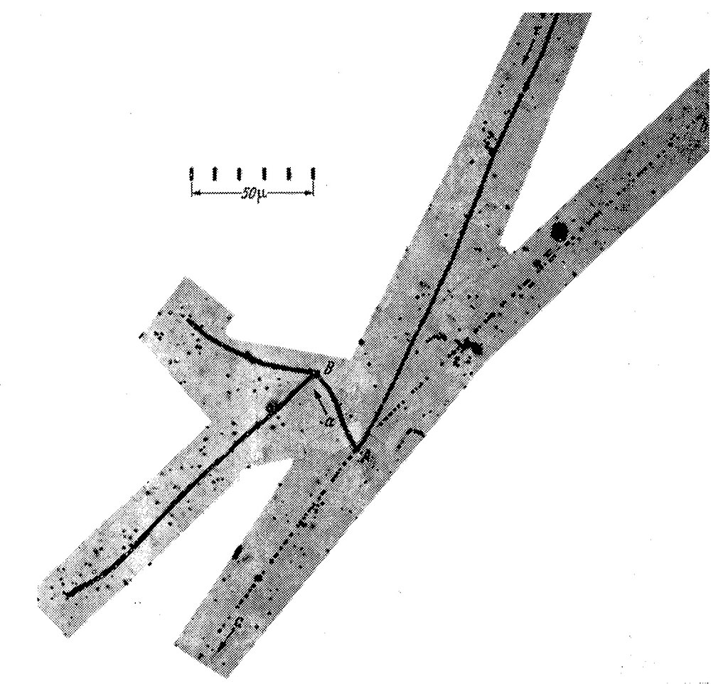
In whatever implementation, particle tracks make the passage of a particle look very particle-like. For example, the image in Fig. WP.1 shows a particle called a kaon initially entering the frame from the top and apparently traveling like a bullet in a straight line, leaving a trace as it moves. Then at some point, the kaon decays into three other particles known as pions, with lines shooting off in three other directions as if the bullet disintegrated into three fragments that go flying off. This seems hard to square with the picture of wave-like behavior. Particularly, at the point of decay (labeled ‘A’ in the figure), the Schrödinger equation would predict a wave function in which the three pions are described by spherically expanding waves, like circular ripples in a pond but in 3D. These waves may have a greater or lesser amplitude in different directions, but certainly not just narrow tracks in three apparently random directions. (And not to overcomplicate things, but the the Schrödinger equation would also not predict a specific, randomly chosen position or time of decay. This topic is discussed in the section Quantum jumps.)
To appreciate the oddness of the 3D particle track, consider a pion initially at point A with a wave function expanding outwards as a spherical wave. As it expands, it encounters a dense 3D array of microscopic detectors that surround it. The wave interacts with the many, many particles within all of the detectors. What we end up seeing though, is just a linear streak of detectors being activated. If we assume that the first detector to be triggered constitutes a collapse-inducing “measurement,” then it would make sense that only the subsequent detectors along a line would be triggered. But the particle might be moving really fast, possibly very close to the speed of light. Does measurement and subsequent collapse happen so fast that it is already complete by the time the second detector is encountered? Certainly there is not time for anything macroscopic to have occurred. So if a “measurement” must involve a macroscopic number of degrees of freedom, do we consider the collapse to occur retroactively?
The solution, again, will be to consider the branching wave function of the particle, detectors, and environment. This explanation was first explored by Mott in 1929, in the early days of quantum mechanics. There, he considered the evolution of the wave function of the incident particle and a series of detectors. Once the particle has passed through, then the detectors can be measured according to the measurement postulate, resulting in a linear track. More recently, Dieter Zeh and other have eliminated the need for a classical measurement at all, describing the whole system and environment in terms of the branching wave function and its many worlds. We’ll see that the detection of particles in the double slit experiment can be understood in a similar way.
Particle tracks
First, let’s take a look at the particle track problem. How can a wave interacting with an array of detectors as it spreads out in all directions show up as a linear track of activated detectors?
We’ll first borrow from the methods and simulations already seen in Catland to reduce the problem to a 1D scenario with wave packets. Then we’ll simulate the case in 2D to get a more realistic picture.
Particle tracks in 1D
In a one dimensional analogy, a 3D spherical wave expanding from a point becomes a superposition of two wave packets both initially at the same position, traveling in opposite directions. We have, in fact, already seen such a scenario back in Fig. 5.1. In that case, the wave packets started out spatially separated and came together, but we can either imagine that process in reverse, or imagine the end of that process as the starting point for the case here where the two packets will then travel apart.
We then wish to place an array of detectors along the line on both sides of the initial packet location. These detectors, with fixed positions, will be activated by the passage of a packet. We have looked at something like this previously, in the point-like two-level detectors used to measure the phase difference between two packets in the section Complementary observables. These detectors could also be used to partially record the passage of a packet, though with imperfect fidelity. Those detectors also caused the incoming packet to split evenly into two packets, one continuing on and one reflected back.
Here, we will use the same sort of model of a detector, but the detector will be affected by the particle from a larger distance (larger than the wave spacing, but still smaller than the packet width). In the Complementary observables section, the range of influence had to be very sharp to measure the phase difference via the interference fringes. If we take the opposite case, where the range of influence is more broad and smooth (as compared to the interference fringe spacing), then the detector will be affected by the passage of the particle, but not sensitive to any phase differences. In this case, we can tune the strength of the interaction so that the detector is completely switched from one state to another by the passage of a packet, with negligible reflection of the packet. (Note: This same sort of position detector is described in section Quantum jumps.)
We could imagine this detector to be an electron bound to an atom. The electron will initially be in its lowest energy orbital – the ground state – which we will denote \(|g\rangle\). As the particle wave packet passes by, the amplitude in the \(|g\rangle\) state begins to transfer to an excited state, denoted \(|e\rangle\). Though the typical case would be that the excited state has a higher energy than the ground state, here we will take the two states to have the same energy. (It doesn’t change much if they have different energies, particularly if the energy difference is small compared to the kinetic energy of the incoming particle.)
First, we will look at how our detector responds to the passage of a generic wave packet. This is simulated in Fig. WP.2. The wave packet is initially at the left, and the detector is in the ground state. This is shown by the fact that the wave function appears in the top panel, correlated with the detector state \(|g\rangle\). As the packet moves past the detector, amplitude is transferred to the lower panel, which shows the part of wave function correlated with detector state \(|e\rangle\). After the wave packet has passed by, there are now two parts to the wave function: in the top panel, the detector remains in \(|g\rangle\) corresponding to an unsuccessful detection of the particle, and in the bottom panel, the detector is now in \(|e\rangle\) corresponding to a detection of the particle. (If we wanted to, we could tune the interaction so as to detect the packet with near-complete success, but it is more realistic to have only a partial chance of success with each interaction.)
In the spirit of simplification, we will first just place a single detector symmetrically on either side of the initial wave packet. The detector on the left starts out in the ground state \(|g\rangle_L\), and likewise the detector on the right starts out in the state \(|g\rangle_R\). We can denote the combined state of both detectors as \(|gg\rangle\), where the first “g” denotes the state of the left detector, and the second “g” denotes the state of the right detector. The initial wave packet is correlated with the state \(|gg\rangle\).
To describe the possible states of the two detectors, we need to make a superposition of four basis states. These four states capture the four independent, distinct states of the pair of detectors. We will use \(|gg\rangle\), \(|ge\rangle\), \(|eg\rangle\), and \(|ee\rangle\). And each of these states may be correlated with a different wave function of the particle. Colloquially, we could say the \(|gg\rangle\) represents neither detector activated, \(|eg\rangle\) or \(|ge\rangle\) represents the left or right detector activated, and \(|ee\rangle\) represents both detectors activated.
Note that \(|gg\rangle\), \(|ge\rangle\), \(|eg\rangle\), and \(|ee\rangle\) are not the only choice of states we could use to describe the two-detector state. For example, we could replace \(|ge\rangle\) and \(|eg\rangle\) with \(|ge\rangle \pm |eg\rangle\), and the math would still work just fine. However, we will argue below that the original proposed choice of basis states is what we will wind up observing macroscopically, so it is useful to look at these particular states from the beginning.
Figure WP.3 shows a simulation of this 1D, two detector scenario. The four frames show the particle waves correlated with \(|gg\rangle\), \(|ge\rangle\), \(|eg\rangle\), and \(|ee\rangle\), with the positions of the two detectors indicated by the dashed lines. Initially, the wave is correlated only with \(|gg\rangle\). One packet travels to the left, eventually interacting with the left detector, and similarly on the right. We see that the packet on the left becomes partially correlated with the state \(|eg\rangle\), and the packet on the right becomes partially correlated with \(|ge\rangle\).
Now we will make a big assumption that won’t be justified for a moment: we will assume that the four panels of Fig. WP.3 can be seen as separate worlds. That is, imagine we have an apparatus with two pointers that can each point to “e” or “g” indicating the state of the two detectors. Then, within the wave function of the universe, there will be parts of it describing different versions of the apparatus indicating each of the four possible outcomes (both “e”, both “g” or one of each). We will argue below that each of these parts of the wave function can be viewed as a separate world, in that henceforth each one will play out as if the others did not exist, at least to a very high degree of accuracy. These different parts of the wave function may have different amplitudes. Recall that we have argued that the amplitudes of the different worlds, or branches of the wave function, can be interpreted as the probability with which we perceive ourselves to become correlated with that world (see Born’s Rule).
With this interpretation, we see what the four versions of the apparatus indicate. The version of the apparatus with both pointers showing “g” is correlated with the \(|gg\rangle\) state of the detectors, and indicates no particle detected. In this part of the wave function, the initial superposition of two wave packets continues on unchanged (i.e. the two packets have equal amplitude.) The version of the apparatus correlated with \(|eg\rangle\) indicates the left detector activated, and only one packet now on the left side past the detector. Likewise, the version that indicates \(|ge\rangle\) sees the right detector activated, only a single packet now past the right detector. And there is no amplitude at all correlated with \(|ee\rangle\): there is essentially no world in which the superposition of packets triggers both detectors.
This simple example already demonstrates the key feature we need to understand so-called wave/particle duality. The initial state of the particle is clearly wave-like. We can even see interference fringes in the initial plot. After the two packets start moving away from each other, the wave of a single electron is now spread over two distinct regions of space – clearly not particle-like behavior. But then the interaction occurs between the electron and the two detectors. This interaction occurs locally. Only the part of the wave on the left interacts with the detector on the left, and becomes correlated with the \(|e\rangle\) state of the left detector, and likewise on the right. Looking just at the waves correlated with \(|eg\rangle\) and \(|ge\rangle\), these waves look a lot more particle-like. Just single wave packets, localized in a single region of space. Though the single wave packets are still somewhat spread out in space, we can sort of get away with thinking of a tiny ball-like particle but with a somewhat uncertain position and velocity. Note that if we try to think of the two-packet state correlated with \(|gg\rangle\) in this picture of classical uncertainty of a ball-like particle, we will quickly run into trouble when those two packets overlap and interfere!
After the apparatus pointer has indicated \(|gg\rangle\), \(|eg\rangle\), or \(|ge\rangle\), a further measurement could be carried out to test for particle- or wave-like behavior. We could reflect both packets back together by placing some reflective wall at the left and right edges of the plots in Fig. WP.3 (now with the detectors removed). Note that the entire wave function is still there, now with three different versions of the apparatus pointers each correlated with their own state of the detectors and original particle. In the part correlated with \(|gg\rangle\), the two packets overlap when they meet and the new measurement could record interference there, as in the Complementary observables section. Clearly wave-like behavior! But in the parts correlated with \(|eg\rangle\) and \(|ge\rangle\), there is only a single packet, so there will be no interference when that packet gets back to the middle. These parts of the wave function, viewed in isolation, would seem to indicate that the detection of the particle on the left or right somehow changed the wave to become particle-like!
Branching
Before going on to more complicated scenarios with more detectors or in two dimensions, let’s think more carefully about how it comes about that that the wave function branches into separate “worlds” here.
The idea of branching is that the wave function of a macroscopic number of particles becomes entangled in such a way that we can divide the wave function up into sufficiently well-separated components such that we can assume they all evolve independently of each other, as if the others did not exist. Recall that the wave function of a macroscopic number of particles exists in a very high dimensional space, something like \(10^{23}\) dimensions. So each “world” is some sort of blob moving about in this configuration space, but the space is so large that we can assume it extremely unlikely that a given blob ever meets another one and interferes. (This picture was described in the section Amplification and decoherence.)
So we are claiming here that the wave function will split up in this way, and that each world will correspond to some combination of the \(|g\rangle\) and \(|e\rangle\) states of the two detectors. We will now discuss why this branching occurs, and why the branches in particular are correlated with the \(|g\rangle\) and \(|e\rangle\) states of a detector, as plotted above. We could have just as well plotted the components correlated with \(|e\rangle + |g\rangle\) and \(|e\rangle - |g\rangle\), by adding and subtracting the two panels.
The answer to this latter question will be:
In order to have macroscopic worlds emerge corresponding to two particular states of a detector like \(|e\rangle\) and \(|g\rangle\), the detector must interact with its environment in a very specific way. (This is sometimes called “einselection,” standing for “environment-induced superselection.”) If the detector interacted with particles in its environment in a different way, it is possible that we would see worlds correlated with a different set of states. Importantly though, there is no guarantee that worlds branch at all. If the interactions with the environment don’t meet the correct conditions, the wave function will just stay unbranched. No one promised that measuring a microscopic quantum system would be easy – it takes a very special system to make it happen.
First, let’s look at what happens when the wave function has not branched. We argued above that following from the end of Fig. WP.3, if we reflect the packets back towards the middle we will see interference correlated with \(|gg\rangle\), but not with \(|eg\rangle\) or \(|ge\rangle\). But now let’s ask, is there any possible way that the packet correlated with \(|eg\rangle\) could ever interfere with the other packet? That is, whatever happens going forward into the future as the particle and detectors interact with everything else in the universe, will it all follow just from that single packet on the left correlated with \(|eg\rangle\), or is it possible that some interference effect would only be understandable if we consider both packets together? [1]
One way that the \(|eg\rangle\) and \(|ge\rangle\) packets can interfere is if future evolution conspires to undo or “erase” the original interaction between particle and detector. Perhaps some further interactions with the environment make it so the detectors work in the reverse direction as they did originally, then the packets are reflected back so they interact with each detector a second time. Or the packets could repeatedly interact with the same detectors so the detector states become rotated all the way back to \(|gg\rangle\). If we had an ideal detector that would flip all the way between \(|g\rangle\) and \(|e\rangle\) when the particle passes by, we would just need two interactions to get everything back to \(|gg\rangle\).
In any case, the point is that such interactions are possible, and in fact reasonably plausible. If we look at just one panel (such as \(|eg\rangle\)) in Fig. WP.3, we cannot justifiably assume that that panel will evolve independently henceforth, with no interference with the packets in other panels. That is, we cannot reasonably view the different panels of the figure as separate worlds.
So how can we get to a situation where we can consider the different detector states \(|gg\rangle\), \(|ge\rangle\), and \(|eg\rangle\) (and possibly \(|ee\rangle\)) to be separate worlds? If the problem with this view is the possibility of undoing the correlations, we just need the correlations to become so elaborate that there is no plausible way for them to be undone. If a macroscopic number of particles also become correlated with these detector states, we would need to undo all of them to see interference starting from the \(|eg\rangle\) or \(|ge\rangle\) packets. It is pretty easy for a macroscopic number of particles to either interact with the detectors, or to interact with other particles that have already interacted with the detectors. There are lots of particles in the environment such as air molecules or photons. In fact, it is quite hard to avoid it, particularly if we hope to amplify the detector state to a macroscopic scale, such as would be needed to move a macroscopic apparatus pointer depending on the detector states. This process of macroscopic correlation, called decoherence, is then essentially inevitable. If, however, we want to be able to distinguish between the \(|e\rangle\) and \(|g\rangle\) states of the detector in particular (as opposed to say \(|e\rangle + |g\rangle\) and \(|e\rangle - |g\rangle\)), then we need these interactions to proceed in a particular way.
Now we will see how we can visualize the decoherence process in the present case. The model of environmental particles will use the same approach as taken in the section Quantum jumps, with some material reproduced here.
We will consider a toy model of a particle in the environment interacting with a detector. We will refer to such a particle as a “probe particle.” The probe particles will initially be described by a single wave packet approaching the detector. The probe particle will interact with the detector in a simple way: if the detector is in the ground state \(|g\rangle\), the probe particle does not interact at all and passes by unaffected; if the detector is in the excited state \(|e\rangle\), the probe particle is strongly repelled at very short distance from the detector and is thus essentially completely reflected. This distinctly different behavior for the \(|g\rangle\) state and \(|e\rangle\) state is what selects this basis for the two worlds that will emerge. The interaction does not cause the detector to shift from \(|g\rangle\) to \(|e\rangle\), and we assume that the probe particle does not interact with original particle at all. Below, we will discuss where this sort of behavior shows up in real physical systems.
Figure WP.4 shows a simulation of the probe particle’s wave function interacting with the detector. For the sake of this example, the detector is initially in a superposition of the ground and excited states, as seen by the nonzero amplitude in both panels. The initial state is not entangled. The probe particle is a single wave packet heading towards the detector, which is separately in a superposition of its two states. After the interaction, however, the state has become entangled. The probe particle has one wave function correlated with the \(|g\rangle\) state of the detector, and a completely different one correlated with \(|e\rangle\). Note that the interaction did not alter the amplitude correlated with \(|g\rangle\) and \(|e\rangle\). In other words, the detector does not “detect” the probe particle.
Now we can return to the case of our particle with two detectors, as shown in Fig. WP.3. What will happen if a probe particle interacts with one of the detectors, say the one on the left? We will see that \(|gg\rangle\) and \(|ge\rangle\) become correlated with the probe particle passing by unaffected (because the left detector is the state “g”), and \(|eg\rangle\) and \(|ee\rangle\) become correlated with the probe particle reflected.
If we want to show this resulting state in the same plot format, each panel must now be a 2D plot to show the wave functions of both the initial particle and the probe particle correlated with the four detector states. This is shown in Fig. WP.5.
At the initial frame of Fig. WP.5, we have the final state of Fig. WP.3 now correlated with a probe particle incoming towards the detector on the left. The horizontal position of the blobs shows the wave function of the original particle correlated with different detector states in each panel. The vertical axis shows the position of the incoming probe particle, which is initially the same for each panel.
As the video in Fig. WP.5 plays, the probe particle is heading towards the detectors. (For simplicity, we have frozen the state of the original particle so it is no longer moving in the horizontal direction.) When the probe particle meets the left detector, the wave function evolves differently in different panels: when the left detector is in the state \(|g\rangle\), the probe particle continues on in the same direction, whereas when the detector is in the state \(|e\rangle\), the probe particle reverses direction.
At the end of the video in Fig. WP.5, we see that the blobs correlated with \(|eg\rangle\) and \(|ge\rangle\) are now separated vertically, in addition to the original horizontal separation. Therefore, if we are ever going to see interference between the two blobs, we would need to undo both the correlation between the original particle and the detector, and the probe particle and the detector.
Now if we imagine \(10^{23}\) probe particles interacting with both detectors in this way, we can see that it would be virtually impossible to ever have the \(|eg\rangle\) and \(|ge\rangle\) blobs interfere with each other. Each probe particle would correspond to a misalignment of the two blobs along a new dimension. Alternatively, we could imagine that the probe particles can also interact with other particles in the environment. So after having interacted with a detector, the transmitted or reflected packet could interact with another particle in the environment. Such interactions can also separate the blobs along new dimensions. This kind of effect even allows for a kind of exponential cascade of correlations to emerge if each probe particle goes on to interact with several other particles, each of which interact with several more particles, and so on.
So the conclusion is: as long as the detectors interact with particles in the environment such that distinctly different states of the environment wind up correlated with the \(|e\rangle\) and \(|g\rangle\) states, then we can safely consider these parts of the wave function as separate worlds.
Particle tracks in a detector array
Having shown how an initial wave function spreading in two directions can result in the activation of a single detector to the left or right, but not both, we can can now extend the picture to a linear array of detectors.
Let’s take one step further: two detectors on each side of the initial particle location. Now with four detectors, there will be 16 distinct detector states. We’ll call them \(|0000\rangle\), \(|0001\rangle\), \(|0010\rangle\), up to \(|1111\rangle\) with all combinations of zeros and ones. Here we have renamed the \(|e\rangle\) and \(|g\rangle\) states of a detector \(|0\rangle\) and \(|1\rangle\).
Therefore, if we want to plot the state of the particle and detectors as we did before, we will need sixteen plots for the parts of the particle wave function correlated with each possible detector state.
Figure WP.6 shows these 16 plots. We are just plotting the real part of the wave function now to avoid overcrowding. Everything else about the simulation is the same as in the two-detector case in Fig. WP.3.
We can see in Fig. WP.6 that only certain detector states wind up correlated with a component of the wave function. Initially, the wave function is correlated with \(|0000\rangle\) corresponding to no detector activated.
The two packets first interact with the inner two detectors, just as they did in the two-detector case in Fig. WP.3. At this point, the largest-amplitude wave function component is still correlated with \(|0000\rangle\), because the passing particle only partially rotates the state of the detector. But we now also have a component correlated with the state \(|0100\rangle\), corresponding to the first left detector activated. This wave function component is just a single packet on the left. Likewise, the component correlated with state \(|0010\rangle\) is just a single packet on the right.
As these three wave function components continue to evolve, we can see what happens following from each individually. When the wave function still correlated with \(|0000\rangle\) interacts with the outer pair of detectors, there is a second chance for a detector to be activated. So again, there is still a substantial amplitude correlated with \(|0000\rangle\), with both packets continuing on. But now there are also components correlated with state \(|1000\rangle\) and state \(|0001\rangle\) which correspond to one of the outer detectors being activated. Each of these detector states is correlated with the single packet following from that detector.
And finally, we see that the parts of the wave function that had become correlated with the inner detectors go on to have a chance to activate both detectors. The components correlated with \(|0100\rangle\) and \(|0010\rangle\) are slightly diminished, while smaller components correlated with \(|1100\rangle\) and \(|0011\rangle\) emerge.
At the end of the video in Fig. WP.6 we see that there are five detector states correlated with a component of the wave function. As before, we argue that once the detectors interact with the environment in the appropriate way, we can consider these different wave function components to be separate worlds.
The worlds that emerge from Fig. WP.6 are just the possible outcomes that we would expect to see in such an experiment, with the probability of each outcome determined by the amplitude of the wave function. The most likely outcome is that no detector is activated, because the detectors are relatively inefficient. In this case, no measurement has occurred and the wave function remains in a superposition of both propagation directions.
But in a world where at least one detector has been activated, we only see activated detectors on one side. Furthermore, in that world, the wave function is now just a single particle-like packet consistent with the side with the activated detectors. And again, because the detectors are not perfect, it is most likely that we see just one detector activated, but it is also possible though with lower probability that we see both detectors activated.
Now we can imagine what would happen with a large number \(N\) detectors on each side. There are now \(2^{2N}\) possible detector states, \(|000 \ldots 0\rangle\) through \(|111 \ldots 1\rangle\). But of these, only states with ones on the left half or right half (or neither) will wind up correlated with components of the wave function. As the packets pass by more and more detectors, the original component correlated with \(|000 \ldots 0\rangle\) will become smaller and smaller. This corresponds to the idea that even though the detectors are imperfect, eventually one will pick up the particle passing by.
So we end up with \(2 \cdot 2^{N} - 1\) different worlds: detector states correlated with some wave function component. One of these is \(|000 \ldots 0\rangle,\) corresponding to the small chance of no detection. Here, no measurement has occurred and the wave function is still a superposition of two now-widely-spaced packets. Another \(2^{N} - 1\) worlds correspond to the \(N\) detectors on just the left having some nonzero number of 1s – a “track” on the left. And the final \(2^{N} - 1\) similarly have 1s on the right – a “track” on the right. Each of these is correlated with just a single wave packet at the left or right.
One can look at the probabilities of these different worlds being observed, following from the amplitudes of the wave packet correlated with each detector state. Each time a packet correlated with some detector state interacts with another detector, its amplitude squared is multiplied by factor \(p<1\), and another component appears correlated with another detector state with amplitude squared \(q=1-p\). The fact that the amplitudes squared must add to one is a mathematical property of the Schrödinger equation. We could think of \(q\) as the probability that the detector is successful in picking up the passage of the particle. As such, the packet correlated with some random detector state \(|11010 \ldots 101\rangle\) will wind up having amplitude squared \(p^{N-m} q^{m},\) where \(m\) is the number of 1’s in the detector state. This becomes particularly simple if \(p=q=1/2\). Then the amplitude squared of the packets correlated with each detector state is the same \((1/2)^{N}\). So we would be equally likely to observe any pattern of activated detectors. But we might be more interested in the question, what is the probability that we observe a certain fraction of activated detectors, without caring about the particular random pattern? This is a standard problem in combinatorics. There is just a single pattern with all \(N\) zeros and another single pattern with all \(N\) ones. There are a great many more random patterns with a 50/50 split of zeros and 1s. The result is that when \(N\) is large, it becomes very likely that we will observe a pattern with a ratio of 1s to zeros close to \(q/p\).
Particle tracks in 2D
So far, we have been looking a simplified 1D picture of particle tracks. The initial wave is expanding outwards in the forward and backward direction. We end up observing either a track going to the left or the right (but not both). In normal situations, however, the waves could be traveling outwards in all three dimensions. As we increase the number of dimensions, the simulations become much more difficult to carry out. But we can still see the relevant effects in a two-dimensional simulation. Due to the difficulty of these simulations, we’ll just look at cases with one detector at a time, so we’ll have to use our imagination a bit to get the real situation.
Figure WP.7 shows an example of a wave expanding outwards in two dimensions. Here we are looking at the amplitude squared of the wave, so we do not see the ripples within the overall expanding circular packet. A detector is positioned at the point indicated by the blue circle. It works the same as the detectors above, but now in 2D. There are two distinct detector states, \(|0\rangle\) and \(|1\rangle\). When the wave gets close to the detector (now in 2D), it causes amplitude to shift between these two states.
As before, the initial wave function is correlated with the detector state \(|0\rangle\). When the wave reaches the detector, we see amplitude begin to be correlated with the \(|1\rangle\) state. The important thing here is that the wave that becomes correlated with \(|1\rangle\) is only shooting off in one direction! We can imagine that if we placed the detector anywhere else around the circle, the wave correlated with \(|1\rangle\) would be downstream of that detector location.
We can put this behavior together with what we saw in the 1D case to imagine a whole ring of \(N\) detectors encircling the initial wave. For simplicity, we will assume that the regions of interaction with each detector do not overlap. Of the total \(2^N\) detector states, we would only see \(N+1\) states correlated with a component of the wave function. The \(|000 \ldots 0\rangle\) state is still correlated with the original circular wave front (reduced in amplitude) representing no detection. And the states with a single 1, such as \(|010 \ldots 0\rangle\) will be correlated with a small wave now localized to be streaming out just from the location of that particular detector.
Now we can place a second ring of detectors beyond the first ring. We can imagine the wave correlated with each state of the first-ring detectors going on to interact with the detectors of the second ring. This is analogous to the four-detector 1D case in Fig. WP.6, when the packets have passed the inner pair of detectors and are about to interact with the outer pair.
By now, the 2D situation with rings of detectors is far too hard to simulate directly. We can, however, look at how the wave correlated with the two detector states of Fig. WP.7 interact with one further detector. The final wave in the \(|0\rangle\) panel of Fig. WP.7 is essentially still just the original expanding circular wave. (The amplitude is slightly reduced in the region where the wave passed the first detector.) This corresponds to no detection in the first ring, and the wave will interact with the second ring in essentially the same way, with some amplitude transferred to the \(|1\rangle\) states of the second ring detectors.
More interesting is the interaction of the wave in the \(|1\rangle\) panel of Fig. WP.7 with detectors in the second ring. Because this wave is preferentially propagating in a particular direction, it will only interact with detectors more or less in line with the first detector. This evolution is shown in Fig. WP.8, where the two panels show the waves correlated with the \(|0\rangle\) and \(|1\rangle\) states of the second detector (both still remain correlated with the \(|1\rangle\) state of the first detector.)
As usual, the top panel of Fig. WP.8 shows the possibility that the wave passes by the detector without triggering it. The bottom panel shows how amplitude is transferred to the \(|1\rangle\) state of this detector when the incoming wave overlaps with it. The resulting wave correlated now with the \(|11\rangle\) state of both detectors again propagates outwards just from the location of the second detector. Of course, we can see that if the detector were moved somewhere to the other side of the figure the wave would not come near it, and there would be no activation of this detector. So just like in the 1D case, multiple detectors can only be activated if they are lined up with each other, forming a “track” of triggered detectors.
One might notice that the waves following from the \(|1\rangle\) states are not propagating in a perfect line – they also spread out sideways. This means that a detector at some small angle from the initial direction could also be triggered. This would show up as a non-straight track. In many realistic cases however, the forward speed of the particle is so great that there isn’t much time for the wave to spread out before encountering the next detector, resulting in very straight tracks [#2]_.
We can now look back at the nuclear emulsion data in Fig. WP.1. The detectors in this case are the photosensitive grains in the emulsion. When the incoming particle decays at point A, the resulting particles are described by expanding spherical waves, akin to the expanding circular wave in Fig. WP.7. As the wave expands it interacts with the nearest grains. There is some amplitude for each grain to be activated. In the part of the wave function correlated with an activated grain, we now see that only grains in the wake of that first grain can be activated. This results in different worlds with tracks of activated detectors in different directions. Moreover, there are also different worlds corresponding to different patterns of activated detectors along the track. Particularly in the less dense tracks in Fig. WP.1, we can see a random appearance of dark spots along a line. The particular direction of the lines, and the particular arrangement of spots along the line will be different in each world. In this world, we observed the particular arrangement of tracks seen in Fig. WP.1.
Double slit experiment
We’ll now return to the familiar double slit experiment. We will see that the apparent wave/particle confusion in this case is resolved in a similar way to that of the particle track scenario.
Unlike the highly simplified 1D model described in the section Double slit, we’ll now look at a less-simplified 2D simulation. This gives us a realistic top-down view of the double slit setup, which is sufficient since nothing very interesting happens along the length of the slits anyway.
Recall the essential particle/wave question in the double slit experiment described above. The parts of an electron’s wave function transmitted through each slit interfere with each other, producing an interference pattern in the wave function when it arrives at a screen. But when we actually detect the position of the electron at the screen, it shows up at a single point. Only when we send in one electron after another do we see the interference pattern build up, because the wave function sets the probability of each detection position.
Figure WP.9 shows a simulation of the Schrödinger equation in a double slit scenario. A 2D wave packet is incoming from left. Again, we are plotting the amplitude squared of the wave function, so we do not see the oscillations of the wave within the packet. The slits are outlined in white, modeled here as a strong potential energy barrier with two openings.
We place our detectors along a vertical line at the right. Due to computational limitations, we can only simulate two detectors at a time indicated by circles in Fig. WP.9. We will have to imagine what it would be like if we had a more dense array of detectors. The detectors here are just the same as in the particle track discussion above. When the wave function comes close to the detector, amplitude is transferred between the \(|0\rangle\) and \(|1\rangle\) states of the detector.
As above, there are four distinct states of the two detectors. In Fig. WP.9 we separately plot the parts of the wave function correlated with the four indicated detector states. The detectors are both initially in the state \(|0\rangle\), so the incoming packet starts out correlated with \(|00\rangle\).
When the packet hits the barrier with the slits, a substantial portion of the wave is reflected. This part is not of particular interest to us. Classically, this would correspond to the situation where the particle just hits the barrier instead of going through a slit, which would be quite likely of course if we are spraying the particles at the barrier randomly.
But we are interested in the case where the particle goes through a slit. Just focusing on the part of the wave that emerges on the right side of the barrier, we can see the expected interference pattern at first correlated with the \(|00\rangle\) state.
When the wave function arrives at the detectors, we see a similar effect to that described in the particle track case. In Fig. WP.9, we have placed the two detectors so they happen to coincide with two maxima of the interference pattern. We see that each detector becomes correlated with a wave with increasing amplitude as the incoming wave passes by. These waves have small amplitude (amplified 25x in the figure to make them visible on the same scale), because we have set the detectors to be fairly inefficient. But the key observations are: 1) we wind up with amplitude correlated with the \(|1\rangle\) state of one detector or the other, but not both; and 2) the wave correlated with each detector state is spatially localized downstream of that detector. This exactly maps onto what we saw in the particle track case. At most one detector is activated, and when it is, the wave correlated with that state acts more “particle-like” in that it is more localized in space in a way consistent with the activation of that detector.
What happens if we place detectors in other positions on the “screen?” Figure WP.10 shows the same simulation, but now one detector is placed near a minimum of the interference, with the other still near a maximum. Now when the wave function interacts with the detectors, the two panels corresponding to activation of one of the detectors become correlated with wave of different amplitudes. In particular, the panel representing activation of the upper detector has only a small amplitude, as that detector is near a minimum of the interference. We interpret the lower amplitude as a lower probability.
From the simulations in Fig. WP.9 and Fig. WP.10, we can imagine what would happen with a dense array of detectors along the screen. With \(N\) detectors, we would require in general \(2^N\) panels to visualize the wave function. After the wave has interacted with the line of detectors, there will be still some smaller amplitude correlated with the state \(|000 \ldots 0\rangle\), corresponding to the possibility that no detector is activated.
Of the remaining possible \(2^N-1\) panels, we only expect to see a wave of any significant amplitude correlated with at most \(N\) of them, corresponding to states with just a single detector activated, and the rest remaining in the \(|0\rangle\) state. (This again assumes that the range of influence of each detector does not overlap its neighbors.)
The wave correlated with each of these \(N\) detector states will have an amplitude that is set by the alignment of that detector with respect to the peaks and troughs of the interference pattern. As before, we assume that the detectors interact with their environment in such a way as to separate the total wave function into separate “worlds.” As was argued in the section Born’s Rule, the amplitude squared of each world yields the probability with which we perceive ourselves to be correlated with that world.
Thus we have \(N+1\) worlds: One in which we see no detector activated, and \(N\) worlds in which we see one of the detectors activated, producing a single “dot” on the screen. We expect to perceive ourself correlated with a world with higher amplitude – more likely to see a detector activated near a peak of the interference, vs. near a trough. Of course, there are now many versions of ourself! Why we assign probabilities to a singular “I” is somewhat mysterious, to say the least (and might be mysterious enough to make some doubt the validity of this whole Many Worlds picture).
Now, starting from each of the \(N+1\) worlds, we can send a second particle through the apparatus. The same thing happens, splitting each world into another \(N+1\) worlds, for a total of \((N+1)^2\) worlds. There is still some amplitude that neither particle has activated a detector. Some worlds will have a single detector activated, either from the first or second particle. And some worlds will now have two detectors activated. Among these worlds, we are more likely to find ourselves correlated with one in which an interference pattern is beginning to emerge: the two activated detectors are most likely near the higher-amplitude regions of the interference pattern.
As more and more particles are sent through the apparatus, we have a proliferation of worlds. These correspond to all possible patterns of activated detectors, one for each particle. Given our assignment of probabilities however, we overwhelmingly expect ourselves to be correlated with a world in which the activated detectors reveal the overall interference pattern.
Which-path redux
Let us now take a quick look again at the which-path effect in the double slit experiment. The two-particle simulations in the Double slit section provided a minimal, 1D illustration of the phenomenon. Here, we can see the same effect in the more realistic 2D simulation. While this scenario makes a clearer connection to the standard double slit geometry, it does hide some of the complexity inside the abstraction of the two-level detector.
Figure WP.11 again shows the 2D double slit scenario, but now with the two detectors placed directly after the slits. As before, there are three detector states correlated with appreciable amplitude in the wave function. The \(|00\rangle\) state, representing no detection, still shows the wave propagating past the slits largely unchanged. In this part of the wave function, the interference pattern appears in the wave function. But the \(|01\rangle\) and \(|10\rangle\) components are only correlated with waves following from one slit or the other. This behavior is the same as above, but now the detectors become correlated with the spatially localized waves before the interference has occurred.
As before, if we assume that the detectors interact with the other particles in the environment so that the wave function components correlated with each of these detector states become very well separated, then we can consider the waves in each panel of Fig. WP.11 to be playing out in separate worlds. In the worlds where a detector registers the passage of the particle, there is no interference.
Real detectors
Above, we have imagined the particle detectors as unspecified degenerate two-level systems. In isolation, there is indeed nothing to distinguish the \(|0\rangle\)/\(|1\rangle\) basis from any another. But not just any two-level system will make a good particle detector. So let’s take a look at some examples of particle detectors.
Perhaps the original particle detector was the cloud chamber, followed later by the bubble chamber, used to observe particle tracks. Both rely on the ionization of atoms by a particle passing through. So in this case, each of our detectors can be viewed as an electron bound to an individual atom. The \(|0\rangle\) state would be the electron in the ground state of the atom, and the \(|1\rangle\) state would be the electron in an unbound state. Clearly, the \(|0\rangle\) and \(|1\rangle\) states will interact with their environment in starkly different ways. Namely, the unbound \(|1\rangle\) state will propagate away from the atom (perhaps as a spherical wave), and scatter off of other particles in the environment. The \(|0\rangle\) state will only be affected by things that can drive atomic transitions. These two states in this basis are distinctly different in their position. As discussed above, this difference can yield interactions that separate the worlds of two basis states, as the interactions typically depend on position.
Other particle detectors rely on excitation of an electron in a semiconductor. An example is another early particle detector, the photographic emulsion. A more modern example would be an avalanche diode. These detectors have been used to observe particle tracks (as shown in Fig. WP.1), and also to register particles coming through a double slit experiment.
In their lowest energy state, the electrons in a semiconductor form an electrically insulating state. That is, they fill all available electron orbitals in a band of energies called the “valence band” such that they are effectively locked in and cannot move. Only a sufficiently energetic kick can knock an electron loose into a higher range of energy states (the “conduction band”) and allow it to move more freely.
A photographic emulsion consists of semiconducting microparticles of silver halides (AgX, where the “X” may stand for a halogen element, chlorine, bromine, iodine, or fluorine). The first step in the detection process is for an incoming particle to excite one or more electrons from the valence band to the conduction band of the AgX particle. So in this case the \(|0\rangle\) state would be the electron in the valence band, and the \(|1\rangle\) state would be the electron in the conduction band. We expect many interactions to affect the electron in the \(|1\rangle\) state, but not the \(|0\rangle\) state. For example, the way the atoms of the crystal vibrate can easily be affected by the electron in the conduction band (so-called “phonon scattering”) but not in the valence band. Or anything else that interacts with the atom via an electric field too weak to kick the valence band electron up to the conduction band can still significantly interact with the electron in the conduction band. This distinctly differnt set of interactions in the \(|1\rangle\) state vs. the \(|0\rangle\) state should effectively split the worlds of the of these two states on a timescale of picoseconds.
In both the cloud/bubble chamber case and the semiconductor case, decoherence (i.e. the well-separation of worlds) seems to happen rather quickly, either by scattering of the electron released by ionization, or by phonon scattering in the conduction band. But even if this didn’t happen, in order to turn these microscopic interactions into a macroscopic effect that we can see with our eyes, further amplification must occur. This generally works by setting off some sort of chain reaction. In the cloud chamber, for example, the ionized atom serves as a nucleation site for condensation to form out of a supersaturated vapor. In the photographic emulsion, the electrons in the conduction band are trapped in defect states, which react with the AgX to form a few atoms of pure Ag. These Ag atoms then serve as a nucleation site for the rest of the particle to convert to pure Ag when placed in a catalyst (the developer). If somehow these systems were to remain coherent after the initial interaction, the amplification to macroscopic scale will almost inevitably split the \(|0\rangle\) and \(|1\rangle\) states into well-separated worlds, due to the position-dependence of interactions.
Footnotes
The answer to this question is
A2. Position space is special because it is where interactions happen locally. We say that two parts of the wave function can be considered separate worlds if they evolve independently. The way that the wave function evolves has two parts: the free evolution corresponding to the particle’s kinetic energy, and forces on the particles due to interactions between particles. It so happens that the forces of nature act in a way that depends on the spatial coordinates of the particles. Therefore, it is interference in position space that affects the interaction force experienced between particles that could affect the evolution of the wave function. If we look at the wave function in momentum space, it is really not that significant if two parts of the wave function overlap in momentum space – it just means that the two parts have the same momentum, even if they are extremely far apart in space. We intuitively know that this has no effect on how the particles behave. If we want to look at how particles interact in momentum space, more complicated mathematical manipulation is required (a convolution of the wave function with a potential function over all space). Position space is where we can see the effect of interactions intuitively by overlap and interference of the wave function components. (Perhaps this is why our brains organize a model of the world in terms of position space!)